Purpose
This project focused on summarizing and replicating the academic paper “Synthetic Control Methods for Comparative Case Studies: Estimating the Effect of California’s Tobacco Control Program” by authors Alberto Abadie, Alexis Diamond, and Jens Hainmueller. This paper utilizes the synthetic control method in order to study the effects of anti-tobacco and smoking legislation passed in 1991 called Proposition 99. This piece of legislation called for a 25 cent increase in California’s existing cigarette tax. Extra revenue generated from this tax was put towards the medical services and anti-tobacco educational campaigns. Such legislation also included “clean-air ordinances” that were implemented throughout the state that banned smoking in the workplace and led municipalities to create ordinance requiring places like restaurants to be 100 percent smoke free.
- Following this, many other states such as Oregon and Arizona passed similar laws that raised the tax levied on cigarettes. At the time of the paper being written, 30 states and 792 municipalities had 100 percent smoke free public spaces.
- While many other previous studies that looked at the effects of regulation on smoking used comparative case studies, this paper utilizes synthetic control to synthesize a fake California counterfactual that represents what would have happened had no proposition 99 been passed and compare the trends between the observed and faked California to see the true effect of the bill on smoking overtime.
- This has the advantage of not being limited to data and groups that were exposed to different levels of smoking regulation and attempts to better create a synthetic control unit.
The causal link that this paper is trying to uncover is the effect of the passage of California’s Proposition 99 in 1988 on tobacco consumption. As with any study or experiment that is trying to get causal effecct, the best method to use is randomized controlled experiments (RCT) in order to get the true causal effect as this method eliminates all selection bias that could mess up the results. To apply that method in this case would be to randomly assign half of a group of participants to smoke before the proposition passed and half to not smoke. Then, you would follow the smokers after the bill passed and compare tobacco consumption between the smokers and non-smokers pre and post-treatment (the passage of Proposition 99 in 1988). However, this is incredibly unethical and impossible to implement because there would be no possibility of an experiment like this being approved or getting funding given the unethical nature of forcing half of the group to smoke cigarettes. Because RCT is not possible, we must use the next best thing available to social scientists: observing what happens in the real world, i.e. natural experiments.
Methodology
As was previously mentioned, the main identification strategy used by the researchers was the synthetic control method. This method uses weights and other similar units, in this case other states, and through assigning weights to the characteristics in question constructs a synthetic (faked) version of California that would represent the trend of tobacco consumption if no proposition 99 was passed. As the authors put it in their paper: “Recall that the synthetic California is constructed as a weighted average of potential control states, with weights chosen so that the resulting synthetic California best reproduces the values of a set of predictors of cigarette consumption in California before the passage of Proposition 99” (Abadie et.al, 2010).
The main assumptions behind a successful synthetic control that must be met are the following:
- Only the treated state is affected by the policy change for all years in the pretreatment period used to create the synthetic control and afterward.
- The policy change has no effect before it is enacted.
- The treated state’s counterfactual outcome can be approximated by a fixed combination of donor states.
The data used in the paper was annual state-level panel data between the years of 1970 and 2000. The pre-treatment period is 1970-1987 and post treatment period is 1988-2000. The variable of interest that is being tracked is annual per-capita cigarette consumption measured in per-capita cigarette sales in packs at the state level. Data was mostly constructed using information on state-level tax revenues on cigarette sales. Relevant variables include the natural long of income, beer consumption, percent of people ages 15-24, cigarette sales, and the retail price of cigarettes.
Analysis Steps
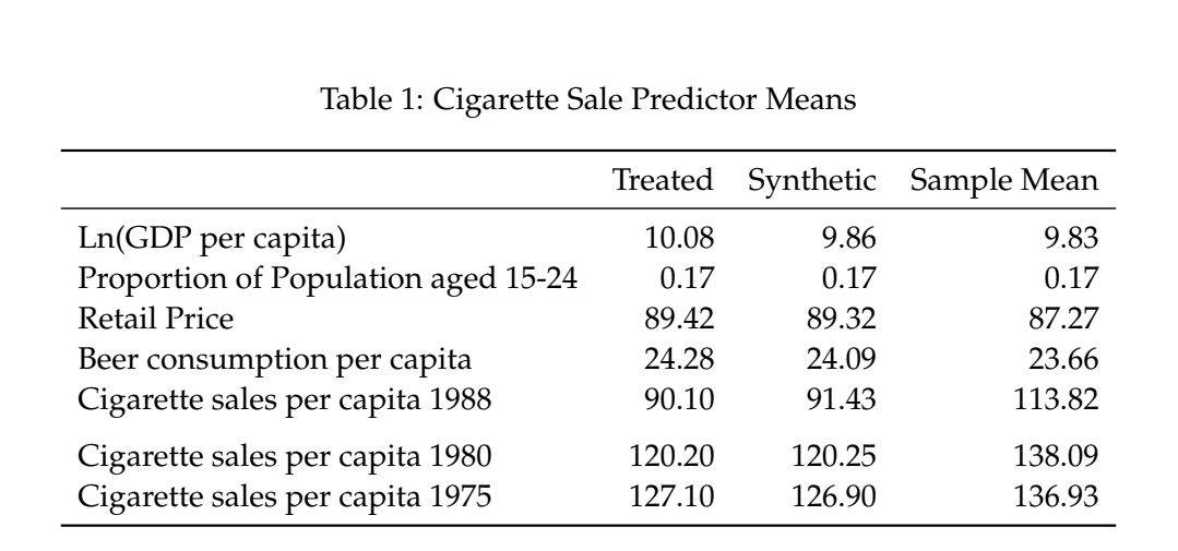
This section will seek to replicate the tables and findings from the original paper using the synthetic control methods. First, we will start with constructing and displaying the balanced table of the cigarette sale indicators that were analyzed in the paper.
1. Cigarette Sale Per Capita Over Time: Preparing the Data
# Calling up the data and packages:
library(tidyverse)
library(Synth)
tobacco_data = readRDS("smoking.RDS")

# Data analysis using Synth:
dataprep.out <-
dataprep(foo = tobacco_data,
       predictors    = c("lnincome","age15to24", "retprice", "beer"),
       predictors.op = "mean",
       time.predictors.prior = 1980:1988,
       dependent     = "cigsale",
       unit.variable = "id",
       unit.names.variable = "state",
       special.predictors = list(
       list("cigsale", 1988, "mean"),
       list("cigsale", 1980, "mean"),
       list("cigsale", 1975, "mean")),
       time.variable = "year",
       treatment.identifier = 3,
       controls.identifier = c(1,2,4:39),
       time.optimize.ssr = 1970:1988,
       time.plot = 1970:2000)
2. Cigarette Sale Per Capita Over Time: Balance Table
# Preparing the Balanced Tables:
synth.out <- synth(dataprep.out)
synth.tables <- synth.tab(dataprep.res = dataprep.out,
                      synth.res = synth.out)

balance<-synth.tables$tab.pred

# Constructing the Balanced Tables:
library(kableExtra)
rownames(balance)<-c("Ln(GDP per capita)","Proportion of Population aged 15-24","Retail Price",
                     "Beer consumption per capita", "Cigarette sales per capita 1988",
                     "Cigarette sales per capita 1980", "Cigarette sales per capita 1975")
kbl(balance, digits=2, caption = "Cigarette Sale Predictor Means", booktabs = T) %>%
kable_styling(bootstrap_options = c("striped", "condensed"))
As we can see from the balanced table below, the treated and synthetic Californias are quite similar to each other in terms of their means for the predictor variables. The values are also quite similar to the overall sample mean, except possibly the lagged cigarette sales per capita, indicating that the weights assigned and the donor data proved to be a good fit in terms of appropriate weights being able to be created. Overall, it seems that based off of this balanced table, the synthetic California is able to match the treated California quite well given the samples provided from the other states and the appropriate weights calculated using the synthetic control method.
3. Cigarette Sale Per Capita Over Time: State Weights Table
# Constructing the weight tables:
weights<-data.frame(synth.tables$tab.w)
weights<-weights%>%select(-unit.numbers)
names(weights)<-c("Weight", "State")
kbl(weights, digits=2, caption = "State weights in the synthetic California", booktabs = T) %>%
kable_styling(bootstrap_options = c("striped", "condensed"))
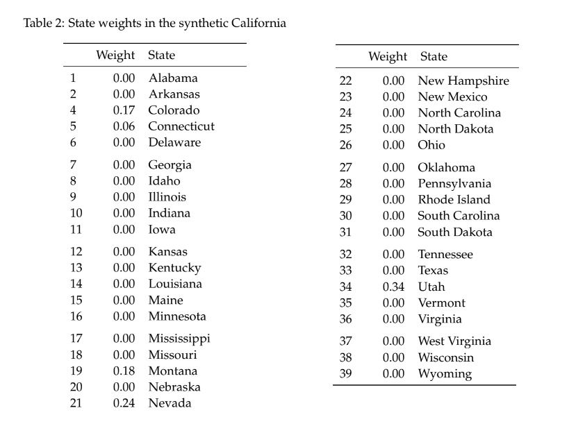
Looking at the weights assigned to the different states above, we see that overall Utah, Nevada, Montana, and Colorado contribute the most to creating the synthetic California, with 0.34, 0.24, 0.18, and 0.17 of the weights, respectively. It’s interesting to see how Utah, despite its somewhat large geographic and cultural difference compared to California contributed its characteristics the most. Nevada is not terribly surprising given its adjacency to California. The rest of the results in terms of weights fall in line with expectations.
4. Cigarette Sale Per Capita Over Time: Trend Plots
# Constructing the trend plots:
path.plot(synth.res = synth.out, dataprep.res = dataprep.out,
      Ylab = "per-capita cigarette sales (in packs)", Xlab = "Year",
      Main = "Figure 2. Trends in per-capita cigarette sales: California vs. synthetic California",
      Ylim = c(0, 140), Legend = c("California","Synthetic California"), Legend.position = "topright",
      tr.intake = 1988)
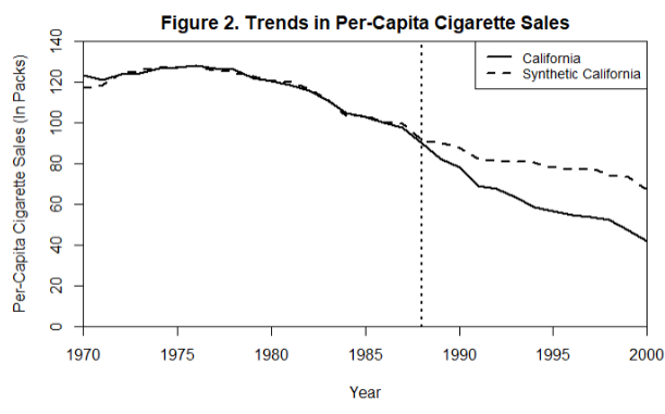
After constructing our trends plot, we note that the trend between synthetic California and treated California prior to the passage of proposition in 1988 are almost identical, meaning that the synthetic California provides a good approximation of a counterfactual of California. From the trend plot, we can see that after the passage of proposition 99 in November of 1988 and its subsequent enactment on the first day of January in 1989,we see that our treated California experiences a decrease from about 90 cigarette sales per capita prior to the passage of proposition 99 to about 40 cigarette sales per capita by 2000. While the synthetic california also depicts a general downward decrease in the number of cigarette sales per capita, the trend plot clearly depicts a wider gap in cigaratte sales per capita compared to the synthetic California created in the previous step. This means that cigarette pack sales fell much faster in the treated California compared to the synthetic version, which ends at roughly 78 cigarette sales per capita by 2000.
5. Cigarette Sale Per Capita Over Time: Gap Plots
# Constructing the gap plots:
gaps.plot(synth.res = synth.out, dataprep.res = dataprep.out,
       Ylab = "gap in per-capita cigarette sales (in packs)", Xlab = "Year",
       Main = "Figure 3. Per-capita cigarette sales gap between California and synthetic California",
      tr.intake = 1988)
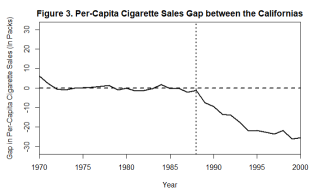
The gap plot confirms our hunch from the previous trend plot, with an over 25 cigarette sale per-capita difference between the treated and synthetic California. As the map depicts, the gap begins to occur right after the passage of proposition 99 and only widens over time with the treated California seeing lower amounts of cigarette sales per-capita compared to the synthetic version. This quite substantial drop in cigarette sales per capita, about 25 percent, visually highlights the large magnitude that proposition 99 had on cigarette sales in California.
6. Cigarette Sale Per Capita Over Time: Placebo Study
# Preparing the placebo plots:
library(SCtools)
placebo <- generate.placebos(dataprep.out = dataprep.out,
synth.out = synth.out, strategy = "multiprocess")
# Constructing the placebo plots:
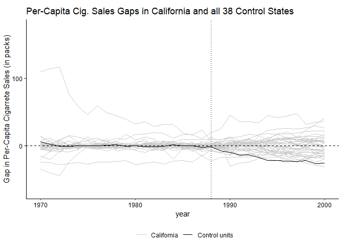
plot_placebos(placebo, title = "Per-capita cigarette sales gaps in Clifornia and placebo gaps in all 38 control states",
ylab = "gap in per-capita cigarrete sales (in packs)", xlab = "year")
We can construct a placebo study in order to compare the estimated effects of proposition 99 on the other states in the donor pool to observe what happens. As the placebo plot depicts below, it seems that the effects of proposition 99 cannot be reproduced in a good manner, most likely due to there being a lack of states in the donor pool that are able to provide characteristics and weights to fit each of the other 38 states that served as controls. The authors bring this issue up in regards to New Hampshire and how it has the highest per capita cigarette sales and no combination of weights from the other states can reproduce the sales observed in New Hampshire. Despite this, the black line, which represents California, is unusually low compared to the other faked placebo trends, indicating that the differences in cigarette sales over time are quite large and stick out compared to the other faked treatments on the other states. These placebo graphs on their own do not provide enough information to estimate whether or not the results are due to chance, so to get that number, we will use a MSPE ratio test to get the exact p-value of this test.
7. Cigarette Sale Per Capita Over Time: MSPE Plot and P-Value
# Constructing the MSPE plot:
mspe.plot(tdf = placebo)
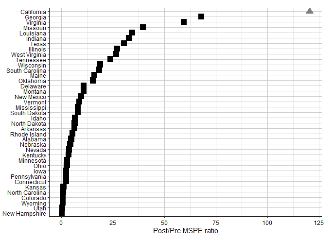
As we can see from the post MSPE / pre MSPE ratio test plot above, California is at the top of the list and has the highest ratio out of all the 39 total states. This large estimated treatment effect for California relative to the placebo effects indicates that the gap between Synthetic and treated California is not due to mere chance and that there is a statistically significant chance that proposition 99 had an effect on the cigarette sales per capita, and thus tobacco consumption, in the state of California follow its passage.
# Calculating the exact p-value:
test_out <- mspe.test(placebo)
test_out$p.val
The exact p-value of our MSPE ratio test is 0.026, meaning that our result is statistically significant at the p = 0.05 threshold. This means that we confirm what our MSPE plot suggested before: the likelihood of observing such a gap between the treated and synthetic Californias is not due to mere chance alone at this significance level.
Overall, the replicated graphs above are quite close to the ones produced in the original paper. Besides some very small differences in the exact numerical values (only off but a couple hundreths of a decimal in most cases), this replication arrives at the same conclusions for all of the major calculations, weights, tables, and figures that the original authors found and I believe this to be a faithful replication overall.
Conclusions and Limitations
In summary, the authors whose analysis has been faithfully replicated above arrived to the conclusion that using the synthetic control method California’s proposition 99 had significant impacts on tobacco consumption (as measured through cigarette sales per capita) following its passage in 1988, with a probability of obtaining these results by chance being extremely small, 0.026. The results found in this paper were much larger than prior estimates that relied on the comparative case study method. In simple terms, both this replication and the original paper conclude that proposition 99 caused a decrease in tobacco consumption in California through its 25 cent raise in the cigarette tax.
In terms of robustness, the placebo test that was constructed delivered mixed results as not all of the donor states had characteristics that could allow for appropriate weights to be constructed once the treatment was faked for each of the other 38 states. Some states observed downwards declines in cigarette sales per capita while others increased. Even after adding and tweaking MSPE cutoffs for the placebo results, the authors found that California still had the largest gap compared to the other placebo gaps of the other states, indicating that our results are quite robust and hold up even under other testing scenarios. Our MSPE plot confirms this, with California at the top with the largest MSPE ratio. Combined with a p-value of 0.026, we can say that our results aren’t due to chance and that the placebo studies conducted in this replication as well as the more extensive plots made in the original paper indicate that our results are robust.
In terms of internal validity, I believe this paper to have successfully identified the causal effect of proposition 99 on tobacco consumption. While using tax revenue from cigarette sales is an imperfect means of measuring consumption as, indicated by the authors, it doesn’t take into account cross-border sales, illicit sales, or other workarounds, the identification strategy itself follows the three main assumptions required for synthetic control to work. Additionally, the synthetic California that was constructed using the other 38 donor states followed the trend in cigarette sales per-capita for the real California up until the treatment in 1988.
- This suggests our synthetic California is a good counter factual to a real California without proposition 99. So internal validity seems strong with this paper.
- In terms of external validity, this was already looked at with the placebo study where we faked the treatment for the other 38 states. Given the mixed results, it seems that some states followed the downward trend in cigarette sales observed in California while others had sales increase.
- Given every states unique populations, cultural, economic, and political structures and norms, it probably is not fair to generalize these results to all states as we saw with New Hampshire's already high cigarette consumption. It could be argued that external validity might be high in more left leaning, democratic states similar to California that have similar progressive agendas. But comparing California to a place like Alabama will probably not work.
Overall, external validity remains low overall and lower than internal validity given the between state differences that exist in this country.